基本规则
copy构造函数是一种特殊的构造函数,函数的名称必须和类名称一致,没有返回值。它必须的一个参数是本类型的一个引用变量,如果形参是对象做值传递, 将实参传进函数时, 我们实际是拷贝一个副本,这样又要调用拷贝构造函数, 层层递归, 会把栈堆满。类中可以存在多个copy构造函数。
编译器会自动生成默认copy构造函数,这个构造函数很简单,仅仅使用“老对象”的数据成员的值对“新对象”的数据成员逐个进行赋值,也就是浅拷贝。
默认copy构造函数不处理静态变量。如果静态成员变量在构造、析构实例的时候需要修改,那么通常需要手工实现copy构造函数和重载赋值运算符。
如果对象存在了动态成员,那么需要手动实现析构函数,也就需要手动实现copy构造函数,因为默认copy构造函数使用的是浅拷贝,要改用深拷贝。
如果派生类没有自定义拷贝构造函数,它在拷贝时,会调用基类的copy构造函数。如果两个类都自定义copy构造函数,那么只调用派生类的。
copy构造函数也要对常成员变量进行列表初始化
基类定义了带参数的构造函数,派生类没有定义任何带参数的构造函数,则不能直接调用基类的带参构造函数,程序编译不通过
深拷贝
浅拷贝实际是对变量的引用,深拷贝是对类成员复制并重新分配内存, 二者的最大区别在于是否手动分配内存
1 | class Base |
不能不处理p。假如copy构造函数中没有对p分配内存,编译正确,但运行时b2析构会出现问题。因为默认拷贝执行浅拷贝,把b2里的p也指向了b1里的p,二者地址相同,结果会出现二次析构,内存泄漏。
我用Creator试验二次析构,发现程序结束时报错 program has unexpectedly finished ,再次运行时Qt先报信息Fault tolerant heap shim applied to current process.,这就是内存泄漏造成的,按照这个方法解决
标准化容器使用insert、push、assign等成员增加元素的时候也会调用拷贝构造函数
禁用拷贝
禁用原因主要是两个:
- 浅拷贝问题,也就是上面提到的二次析构。
- 自定义了基类和派生类的copy构造函数,但派生类对象拷贝时,调用了派生类的拷贝,没有调用自定义的基类拷贝而是调用默认的基类拷贝。这样可能造成不安全,比如出现二次析构问题时,因为不会调用我们自定义的基类深拷贝,还是默认的浅拷贝。
Effective C++条款6规定,如果不想用编译器自动生成的函数,就应该明确拒绝。方法一般有三种:
- C++11对函数声明加delete关键字:
Base(const Base& obj) = delete;,不必有函数体,这时再调用拷贝构造会报错 - 最简单的方法是将copy构造函数声明为private
- 条款6给出了更好的处理方法:创建一个基类,声明copy构造函数,但访问权限是private,使用的类都继承自这个基类。默认copy构造函数会自动调用基类的copy构造函数,而基类的copy构造函数是private,那么它无法访问,也就无法正常生成copy构造函数。
Qt就是这样做的,QObject定义中有这样一段,三条都利用了:1
2
3
4
5
6private:
Q_DISABLE_COPY(QMainWindow)
类的不可拷贝特性是可以继承的,凡是继承自QObject的类都不能使用copy构造函数和赋值运算符
如果一个类的拷贝构造函数加了delete关键字,类名就不能作为函数的形参,可以改用指针或const引用
有没有定义派生类copy构造函数的情况的不同结果
先是没有定义派生类copy构造函数的情况:1
2Derived f;
Derived ff(f);
运行结果是这样:1
2
3
4
5
6
7
8Base constrct 0x75fd20
Derived construct 0x75fd20
Base copy constrct 0x75fd10
*************
Derived deconstruct 0x75fd10
Base deconstrct 0x75fd10
Derived deconstruct 0x75fd20
Base deconstrct 0x75fd20
对于副本的对象,只调用了基类copy构造函数。
然后是定义的情况,运行结果是这样: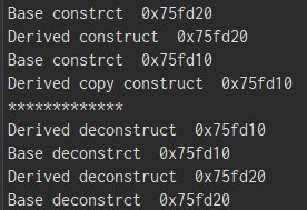
先是f的基类构造和派生类构造,然后进入ff,这里的对象是个副本,所以this指针的地址不同了, 先是基类构造然后是派生类拷贝构造, 销毁时倒没什么特别。
这样看来, 派生类的copy构造函数可以尽量不定义。