类的定义1
2
3
4
5
6
7
8
9
10
11
12
13
14
15
16
17
18
19
20
21
22
23
24
25
26
27
28
29
30
31
32
33
34
35
36
37
38
39
40
41
42
43
44
45
46
47
48
49
50
51
52
53
54
55
56
57
58
59
60
61
62
63
64
65
66
67
68
69
70
71
72
73
74
75
76
77
78
79
80
81
82
83
84
85
86
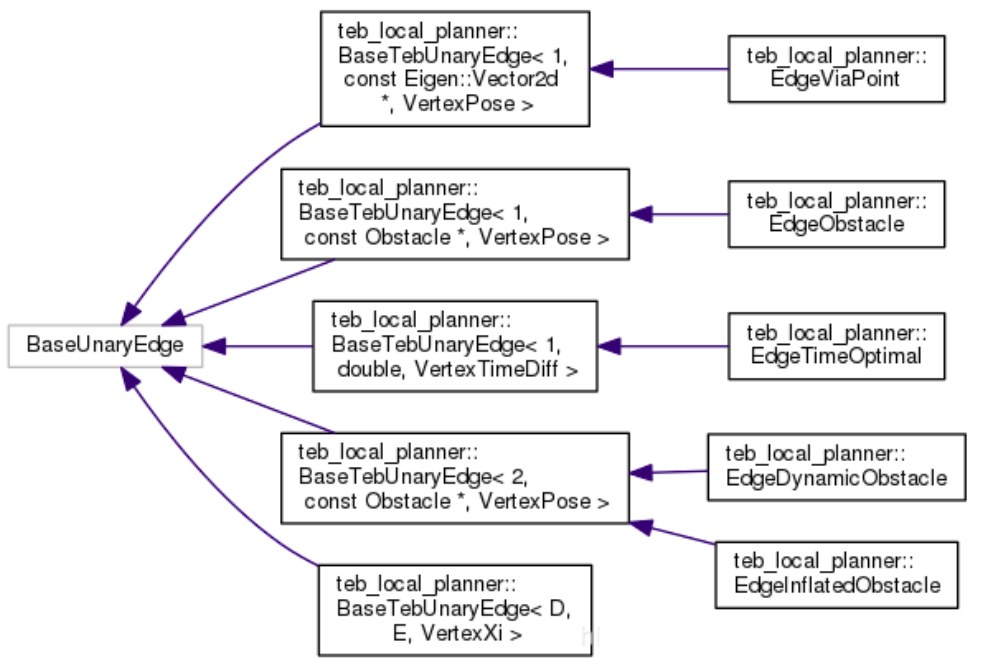
87/**
* Edge defining the cost function for keeping a minimum distance from obstacles.
* The edge depends on a single vertex \f$ \mathbf{s}_i \f$ and minimizes:
* \f$ \min \textrm{penaltyBelow}( dist2point ) \cdot weight \f$.
* \e dist2point denotes the minimum distance to the point obstacle.
* \e weight can be set using setInformation(). \n
* \e penaltyBelow denotes the penalty function, see penaltyBoundFromBelow()
* @see TebOptimalPlanner::AddEdgesObstacles, TebOptimalPlanner::EdgeInflatedObstacle
* @remarks Do not forget to call setTebConfig() and setObstacle()
*/
class EdgeObstacle : public BaseTebUnaryEdge<1, const Obstacle*, VertexPose>
{
public:
EdgeObstacle()
{
_measurement = NULL;
}
/**
* @brief Set pointer to associated obstacle for the underlying cost function
* @param obstacle 2D position vector containing the position of the obstacle
*/
void setObstacle(const Obstacle* obstacle)
{
_measurement = obstacle;
}
/**
* @brief Set pointer to the robot model
* @param robot_model Robot model required for distance calculation
*/
void setRobotModel(const BaseRobotFootprintModel* robot_model)
{
robot_model_ = robot_model;
}
/**
* @brief Set all parameters at once
* @param cfg TebConfig class
* @param robot_model Robot model required for distance calculation
* @param obstacle 2D position vector containing the position of the obstacle
*/
void setParameters(const TebConfig& cfg,
const BaseRobotFootprintModel* robot_model, const Obstacle* obstacle)
{
cfg_ = &cfg;
robot_model_ = robot_model;
_measurement = obstacle;
}
// cost function
void computeError()
{
ROS_ASSERT_MSG(cfg_ && _measurement && robot_model_, "You must call setTebConfig(), setObstacle() and setRobotModel() on EdgeObstacle()" );
const VertexPose* bandpt = static_cast<const VertexPose*>(_vertices[0]);
/* inline double penaltyBoundFromBelow( const double& var,
const double& a, const double& epsilon)
{
if (var >= a+epsilon)
return 0.;
else
return (-var + (a+epsilon));
} */
double dist = robot_model_->calculateDistance(bandpt->pose(), _measurement);
// Original obstacle cost
_error[0] = penaltyBoundFromBelow( dist,
cfg_->obstacles.min_obstacle_dist,
cfg_->optim.penalty_epsilon );
if (cfg_->optim.obstacle_cost_exponent != 1.0 && cfg_->obstacles.min_obstacle_dist > 0.0)
{
// Optional non-linear cost. Note the max cost (before weighting) is
// the same as the straight line version and that all other costs are
// below the straight line (for positive exponent), so it may be
// necessary to increase weight_obstacle and/or the inflation_weight
// when using larger exponents
_error[0] = cfg_->obstacles.min_obstacle_dist * std::pow(
_error[0] / cfg_->obstacles.min_obstacle_dist,
cfg_->optim.obstacle_cost_exponent);
}
ROS_ASSERT_MSG(std::isfinite(_error[0]),
"EdgeObstacle::computeError() _error[0]=%f\n",
_error[0]);
}
protected:
const BaseRobotFootprintModel* robot_model_;
public:
EIGEN_MAKE_ALIGNED_OPERATOR_NEW
};
一元边,观测值维度为1,测量值类型为Obstacle基类,连接VertexPose顶点。存储了某个障碍物的中心点的三维位置,形状与顶点的位置
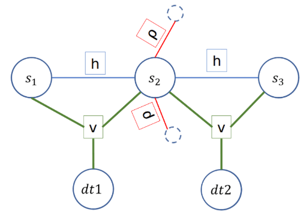
只将离某个Pose最近的最左边与最右边的两个Obstacle加入优化中。(因为优化路径不会使得路径相对于障碍物的位置关系发生改变)。同时,还设了一个阈值,凡是离该Pose距离低于某个距离的障碍物也一并加入考虑之中。1
2
3
4
5
6
7
8
9
10
11
12
13
14
15
16
17
18
19
20
21
22
23
24
25
26
27
28
29
30
31
32
33
34
35
36
37
38
39
40
41
42
43
44
45
46
47
48
49
50
51
52
53
54
55
56
57
58
59
60
61
62
63
64
65
66
67
68
69
70
71
72
73
74
75
76
77
78
79
80
81
82
83
84
85
86
87
88
89
90
91
92
93
94
95
96
97
98
99
100
101
102
103
104
105
106
107
108
109void TebOptimalPlanner::AddEdgesObstacles(double weight_multiplier)
{
if (cfg_->optim.weight_obstacle==0 || weight_multiplier==0 || obstacles_==nullptr )
return;
// 判断 inflation_dist > min_obstacle_dist
bool inflated = cfg_->obstacles.inflation_dist > cfg_->obstacles.min_obstacle_dist;
Eigen::Matrix<double,1,1> information;
information.fill(cfg_->optim.weight_obstacle * weight_multiplier);
Eigen::Matrix<double,2,2> information_inflated;
information_inflated(0,0) = cfg_->optim.weight_obstacle * weight_multiplier;
information_inflated(1,1) = cfg_->optim.weight_inflation;
information_inflated(0,1) = information_inflated(1,0) = 0;
auto iter_obstacle = obstacles_per_vertex_.begin();
auto create_edge = [inflated, &information, &information_inflated, this] (int index,
const Obstacle* obstacle) {
if (inflated)
{
// 一元边,观测值维度为2,类型为Obstacle基类,连接VertexPose顶点
EdgeInflatedObstacle* dist_bandpt_obst = new EdgeInflatedObstacle;
dist_bandpt_obst->setVertex(0,teb_.PoseVertex(index));
// 信息矩阵为2x2对角阵,(0,0) = weight_obstacle, (1,1) = weight_inflation
dist_bandpt_obst->setInformation(information_inflated);
dist_bandpt_obst->setParameters(*cfg_, robot_model_.get(), obstacle);
optimizer_->addEdge(dist_bandpt_obst);
}
else
{
// 一元边,观测值维度为1,测量值类型为Obstacle基类,连接VertexPose顶点
EdgeObstacle* dist_bandpt_obst = new EdgeObstacle;
dist_bandpt_obst->setVertex(0,teb_.PoseVertex(index));
// 信息矩阵为 1x1 weight_obstacle * weight_multiplier
dist_bandpt_obst->setInformation(information);
dist_bandpt_obst->setParameters(*cfg_, robot_model_.get(), obstacle);
optimizer_->addEdge(dist_bandpt_obst);
};
};
/* iterate all teb points, skipping the last and, if the
EdgeVelocityObstacleRatio edges should not be created, the first one too*/
const int first_vertex = cfg_->optim.weight_velocity_obstacle_ratio == 0 ? 1 : 0;
for (int i = first_vertex; i < teb_.sizePoses() - 1; ++i)
{
double left_min_dist = std::numeric_limits<double>::max();
double right_min_dist = std::numeric_limits<double>::max();
ObstaclePtr left_obstacle;
ObstaclePtr right_obstacle;
const Eigen::Vector2d pose_orient = teb_.Pose(i).orientationUnitVec();
// iterate obstacles
for (const ObstaclePtr& obst : *obstacles_)
{
// we handle dynamic obstacles differently below
if(cfg_->obstacles.include_dynamic_obstacles && obst->isDynamic())
continue;
// calculate distance to robot model
double dist = robot_model_->calculateDistance(teb_.Pose(i), obst.get());
// force considering obstacle if really close to the current pose
if (dist < cfg_->obstacles.min_obstacle_dist*cfg_->obstacles.obstacle_association_force_inclusion_factor)
{
iter_obstacle->push_back(obst);
continue;
}
// cut-off distance
if (dist > cfg_->obstacles.min_obstacle_dist*cfg_->obstacles.obstacle_association_cutoff_factor)
continue;
// determine side (left or right) and assign obstacle if closer than the previous one
if (cross2d(pose_orient, obst->getCentroid()) > 0) // left
{
if (dist < left_min_dist)
{
left_min_dist = dist;
left_obstacle = obst;
}
}
else
{
if (dist < right_min_dist)
{
right_min_dist = dist;
right_obstacle = obst;
}
}
}
// create obstacle edges
if (left_obstacle)
iter_obstacle->push_back(left_obstacle);
if (right_obstacle)
iter_obstacle->push_back(right_obstacle);
// continue here to ignore obstacles for the first pose, but use them later to create the EdgeVelocityObstacleRatio edges
if (i == 0)
{
++iter_obstacle;
continue;
}
// create obstacle edges
for (const ObstaclePtr obst : *iter_obstacle)
create_edge(i, obst.get());
++iter_obstacle;
}
}
误差函数的计算
两个类根据机器人的轮廓模型计算当前Pose与某个障碍物的距离dist,至于如何计算,属于另一个话题。 然后EdgeObstacle的error如下1
error = (dist > min_obstacle_dist+ε) ? 0 : (min_obstacle_dist+ε) - dist
EdgeInflatedObstacle则是1
2
3
4# Original "straight line" obstacle cost. The max possible value
# before weighting is min_obstacle_dist,和 EdgeObstacle的相同
error[0] = (dist > min_obstacle_dist+ε) ? 0 : (min_obstacle_dist+ε) - dist
error[1] = (dist > inflation_dist) ? 0 : (inflation_dist) - dist
但是这两个类的computeError在error[0]赋值结束后又补充这样一段:1
2
3
4
5
6
7
8
9
10if (cfg_->optim.obstacle_cost_exponent != 1.0 && cfg_->obstacles.min_obstacle_dist > 0.0)
{
/* Optional 非线性代价. Note the max cost (before weighting) is
the same as the straight line version and that all other costs are
below the straight line (for positive exponent), so it may be
necessary to increase weight_obstacle and/or the inflation_weight
when using larger exponents */
_error[0] = cfg_->obstacles.min_obstacle_dist * std::pow(
_error[0] / cfg_->obstacles.min_obstacle_dist, cfg_->optim.obstacle_cost_exponent);
}
涉及参数obstacle_cost_exponent,不明白这个公式是怎么来的