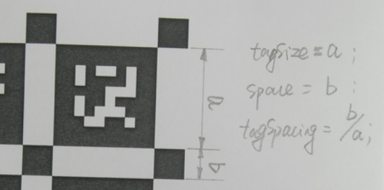
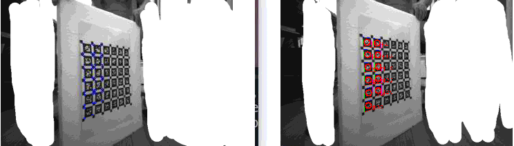
target_type: 'aprilgrid'#gridtype tagCols: 6 #number of apriltags tagRows: 6 #number of apriltags tagSize: 0.035 #size of apriltag, edge to edge [m] tagSpacing: 0.3 #ratio of space between tags to tagSize
A ROS package tool to analyze the IMU performance. C++ version of Allan Variance Tool. The figures are drawn by Matlab, in scripts.
Actually, just analyze the Allan Variance for the IMU data. Collect the data while the IMU is Stationary, with a two hours duration. code_utils标定IMU的噪音密度和随机游走系数。
The following packages have unmet dependencies:
 libdw-dev : Depends: libelf-dev but it is not going to be installed
             Depends: libdw1 (= 0.165-3ubuntu1) but it is not going to be installed
E: Unable to correct problems, you have held broken packages.
这是因为一个依赖项已经安装了不同版本:Depends: libelf1 (= 0.165-3ubuntu1) but 0.165-3ubuntu1.2 is to be installed。 解决方法: sudo aptitude install libdw-dev,对给出的方案,选择第二个,降级 libelf1[0.165-3ubuntu1.1 (now) -> 0.158-0ubuntu]
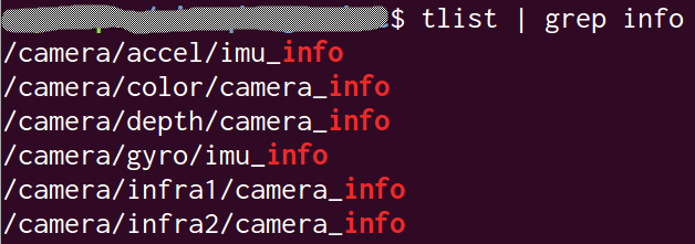
启动: roslaunch realsense2_camera rs_imu_calibration.launch,然后录制imu数据包rosbag record -O imu_calibration /camera/imu,让IMU静止不动两个小时,录制IMU的bag.
标定
根据imu_utils文件夹里面的A3.launch改写D435i标定启动文件:d435i_imu_calib.launch注意,记得修改max_time_min对应的参数,默认是120,也就是两个小时,如果ros包里的imu数据长度没有两个小时,等bag播放完了,还是停留在wait for imu data这里,不会生成标定文件。我录了1小时59分多一点,所以还得改成119
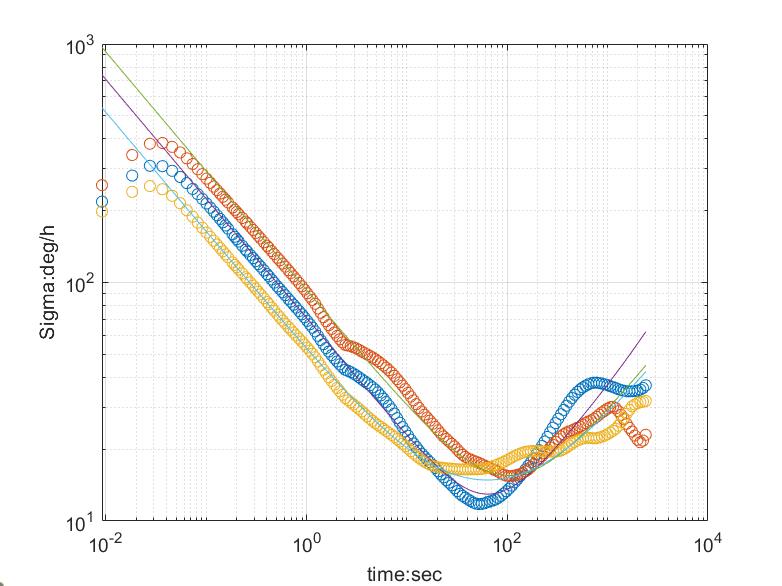
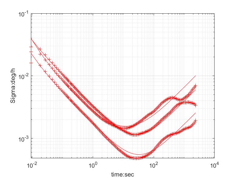
gyr x  numData 781205
gyr x  start_t 1.59343e+09
gyr x  end_t 1.59344e+09
gyr x dt
-------------7140.59 s
-------------119.01 min
-------------1.9835 h
gyr x  freq 109.403
gyr x  period 0.00914049
gyr y  numData 781205
gyr y  start_t 1.59343e+09
gyr y  end_t 1.59344e+09
gyr y dt
-------------7140.59 s
-------------119.01 min
-------------1.9835 h
gyr y  freq 109.403
gyr y  period 0.00914049
gyr z  numData 781205
gyr z  start_t 1.59343e+09
gyr z  end_t 1.59344e+09
gyr z dt
-------------7140.59 s
-------------119.01 min
-------------1.9835 h
gyr z  freq 109.403
gyr z  period 0.00914049
Gyro X
C   -6.83161    94.2973   -19.0588      2.983 -0.0404918
 Bias Instability 2.37767e-05 rad/s
 Bias Instability 6.28462e-05 rad/s, at 63.1334 s
 White Noise 12.9453 rad/s
 White Noise 0.00360015 rad/s
  bias -0.363298 degree/s
-------------------
Gyro y
C   -8.74367    117.584   -15.9277    2.47408 -0.0373467
 Bias Instability 6.41864e-05 rad/s
 Bias Instability 7.52073e-05 rad/s, at 104.256 s
 White Noise 16.8998 rad/s
 White Noise 0.00471573 rad/s
  bias -0.544767 degree/s
-------------------
Gyro z
C   -4.51808    68.1919   -9.33284    1.95333 -0.0262641
 Bias Instability 8.50869e-05 rad/s
 Bias Instability 7.19998e-05 rad/s, at 63.1334 s
 White Noise 9.43212 rad/s
 White Noise 0.00268623 rad/s
  bias -0.0762471 degree/s
-------------------
==============================================
==============================================
acc x  numData 781205
acc x  start_t 1.59343e+09
acc x  end_t 1.59344e+09
acc x dt
-------------7140.59 s
-------------119.01 min
-------------1.9835 h
acc x  freq 109.403
acc x  period 0.00914049
acc y  numData 781205
acc y  start_t 1.59343e+09
acc y  end_t 1.59344e+09
acc y dt
-------------7140.59 s
-------------119.01 min
-------------1.9835 h
acc y  freq 109.403
acc y  period 0.00914049
acc z  numData 781205
acc z  start_t 1.59343e+09
acc z  end_t 1.59344e+09
acc z dt
-------------7140.59 s
-------------119.01 min
-------------1.9835 h
acc z  freq 109.403
acc z  period 0.00914049
acc X
C  3.36177e-05   0.00175435 -0.000159698  7.23303e-05 -7.16006e-07
 Bias Instability 0.000553948 m/s^2
 White Noise 0.018272 m/s^2
-------------------
acc y
C  9.36955e-05   0.00234733   0.00012197  0.000243676 -2.66252e-06
 Bias Instability 0.00156748 m/s^2
 White Noise 0.0289241 m/s^2
-------------------
acc z
C  5.07832e-05   0.00331104 -0.000381222  0.000199602 -2.43776e-06
 Bias Instability 0.00115308 m/s^2
 White Noise 0.0351134 m/s^2
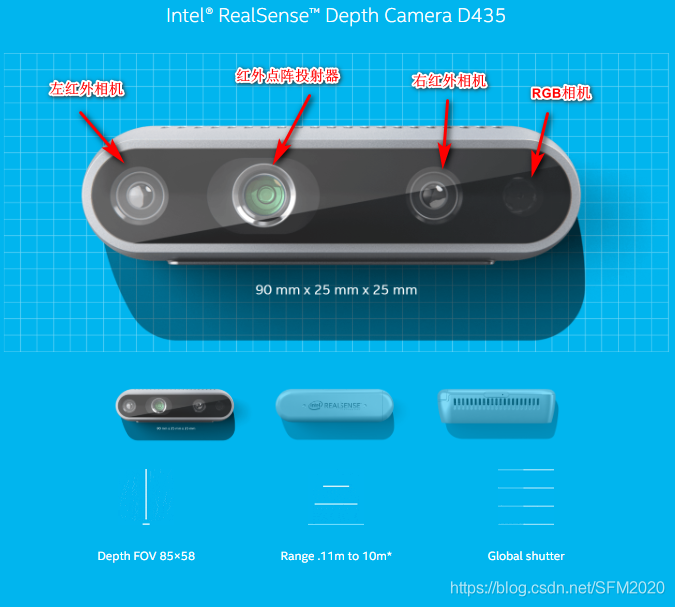
Principal Point         : 327.438, 239.997
Focal Length            : 611.354, 610.016
Distortion Model        : Inverse Brown Conrady
Distortion Coefficients : [0,0,0,0,0]
疑难问题 undefined symbol: _ZN2cv3MatC1Ev
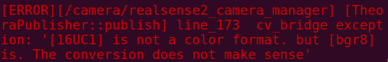
运行rs_camera.launch时报错
1
symbol lookup error: /home/jetson/catkin_ws/devel/lib//librealsense2_camera.so: undefined symbol: _ZN2cv3MatC1Ev [camera/realsense2_camera_manager-2] process has died
RealSense ROS v2.3.2 [ INFO] [1723892537.013079361]: Built with LibRealSense v2.50.0 [ INFO] [1723892537.013109698]: Running with LibRealSense v2.50.0 [ INFO] [1723892537.311113159]: Device with serial number 014122072296 was found. [ INFO] [1723892537.311624883]: Device with physical ID 2-1.4-6 was found. [ INFO] [1723892537.311852281]: Device with name Intel RealSense D435I was found. [ INFO] [1723892537.313360062]: Device with port number 2-1.4 was found. [ INFO] [1723892537.313859786]: Device USB type: 3.2
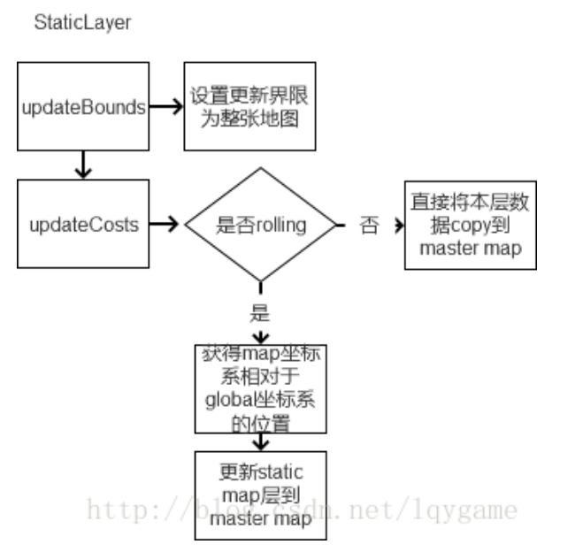
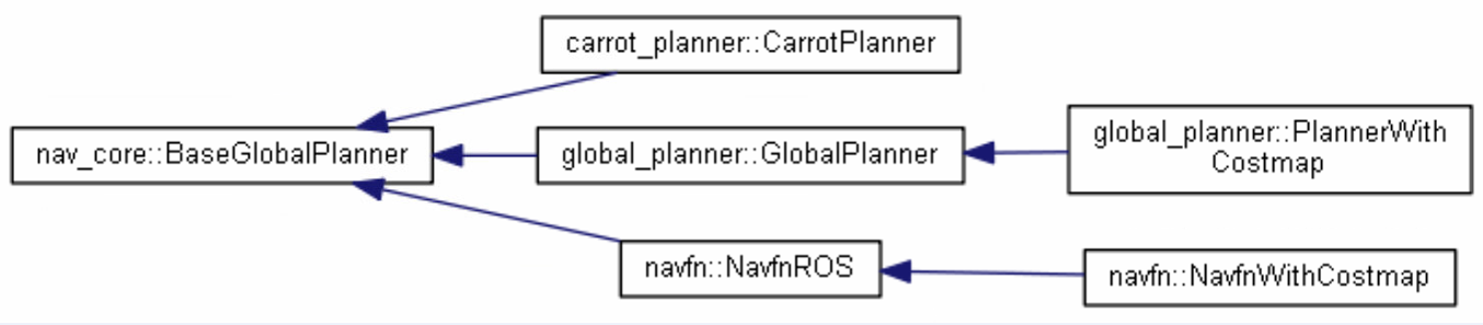
<librarypath="lib/libglobal_planner"> <classname="global_planner/GlobalPlanner"type="global_planner::GlobalPlanner"base_class_type="nav_core::BaseGlobalPlanner"> <description> A implementation of a grid based planner using Dijkstras or A* </description> </class> </library>
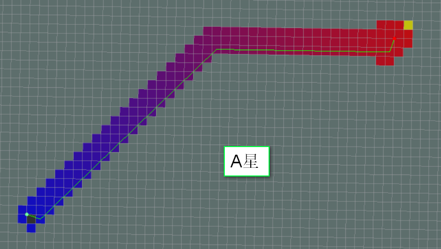
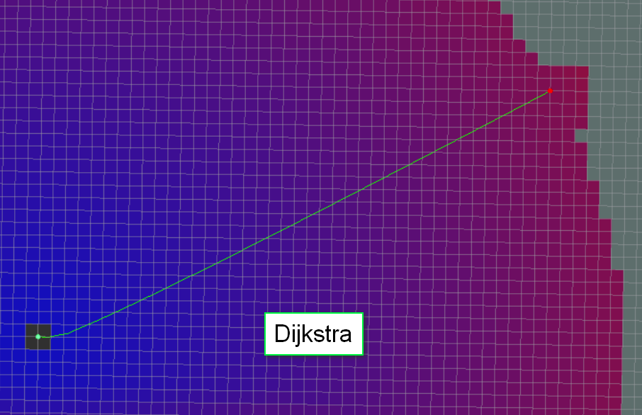
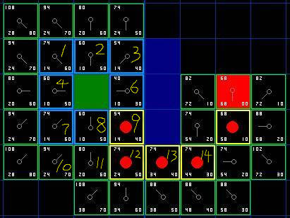
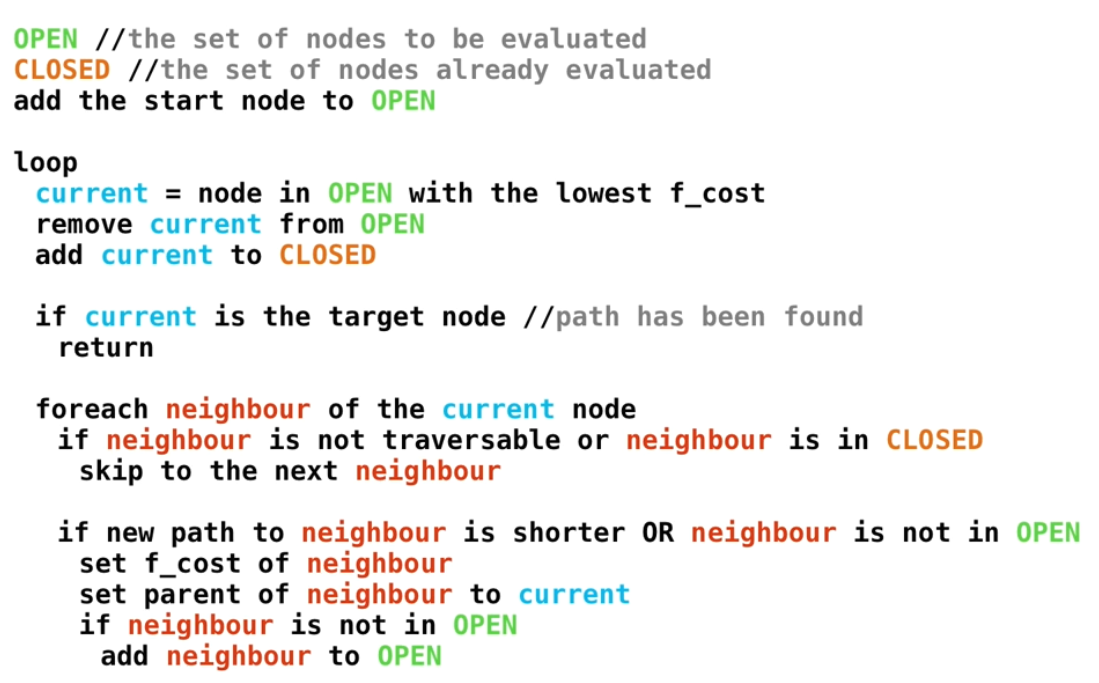
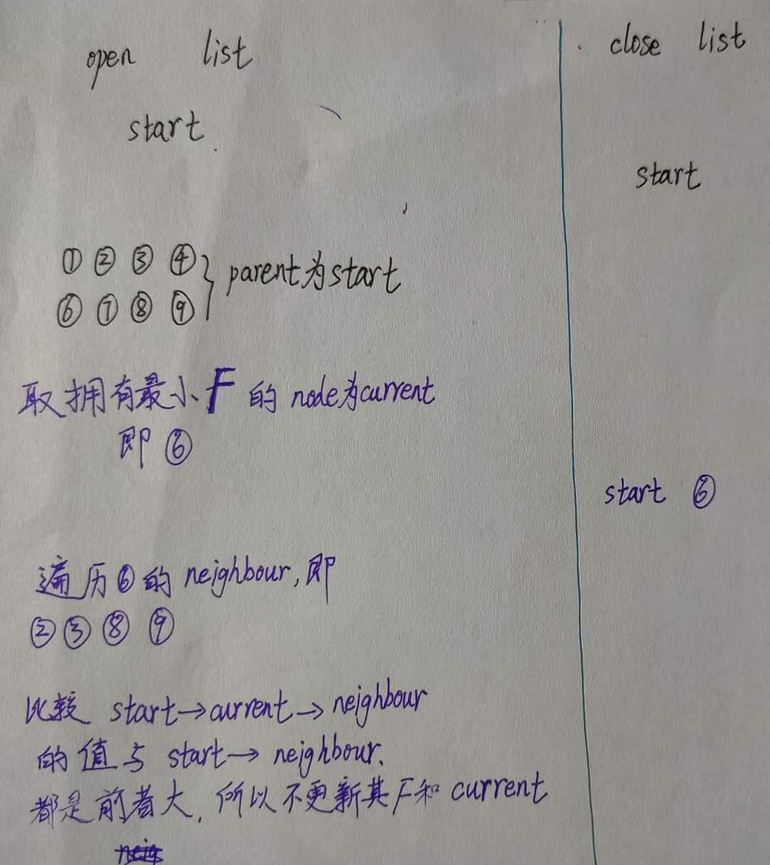
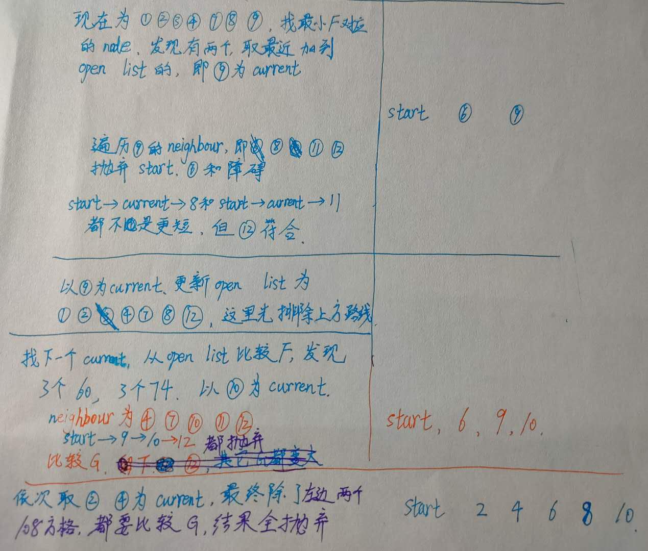
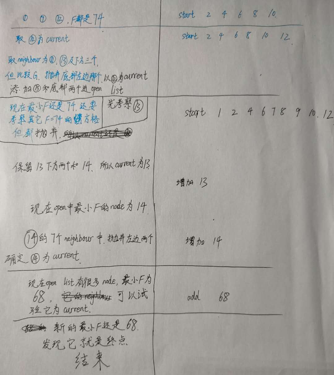
A*比Dijkstra少计算很多,但可能不会产生相同路径。另外,在global_planner的A*里,the potentials are computed using 4-connected grid squares, while the path found by tracing the potential gradient from the goal back to the start uses the same grid in an 8-connected fashion. Thus, the actual path found may not be fully optimal in an 8-connected sense. (Also, no visited-state set is tracked while computing potentials, as in a more typical A* implementation, because such is unnecessary for 4-connected grids).