牛顿法的思路是将函数 f 在 x 处展开为多元二次函数,再通过求解二次函数最小值的方法得到本次迭代的下降方向。那么问题来了,多元二次函数在梯度为0的地方一定存在最小值么?直觉告诉我们是不一定的。以一元二次函数 g(x)=ax2+bx+c为例,我们知道当a>0时,g(x)可以取得最小值,否则g(x)不存在最小值。
if (polygon->points.size()==1 && obstacle->radius > 0) // Circle { obstacles_.push_back(ObstaclePtr(newCircularObstacle(polygon->points[0].x, polygon->points[0].y, obstacle->radius))); } elseif (polygon->points.size()==1) // Point { obstacles_.push_back(ObstaclePtr(newPointObstacle(polygon->points[0].x, polygon->points[0].y))); } elseif (polygon->points.size()==2) // Line { obstacles_.push_back(ObstaclePtr(newLineObstacle(polygon->points[0].x, polygon->points[0].y, polygon->points[1].x, polygon->points[1].y ))); } elseif (polygon->points.size()>2) // Real polygon { PolygonObstacle* polyobst = new PolygonObstacle; for (std::size_t j=0; j<polygon->points.size(); ++j) { polyobst->pushBackVertex(polygon->points[j].x, polygon->points[j].y); } polyobst->finalizePolygon(); obstacles_.push_back(ObstaclePtr(polyobst)); }
// Set velocity, if obstacle is moving if(!obstacles_.empty()) obstacles_.back()->setCentroidVelocity(obstacles->obstacles[i].velocities, obstacles->obstacles[i].orientation); } }
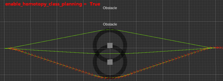
teb_markers (visualization_msgs/Marker) teb_local_planner通过具有不同名称空间的标记来提供规划场景的其他信息。 Namespaces PointObstacles and PolyObstacles: visualize all point and polygon obstacles that are currently considered during optimization. Namespace TebContainer: Visualize all found and optimized trajectories that rest in alternative topologies (only if parallel planning is enabled). Some more information is published such as the optimization footprint model
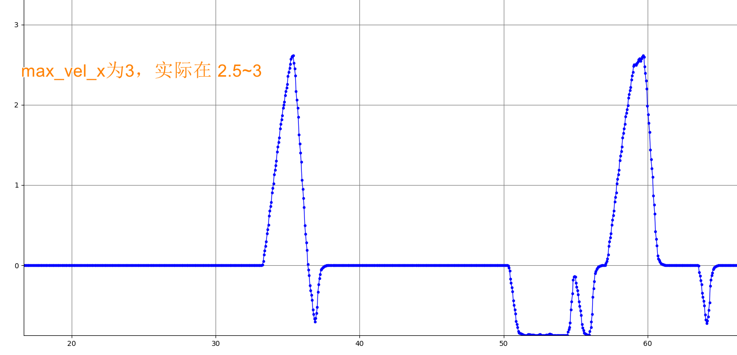
dt_ref: 0.3 局部路径规划的解析度; Temporal resolution of the planned trajectory (usually it is set to the magnitude of the 1/control_rate)。 TEB通过状态搜索树寻找最优路径,而dt_ref则是最优路径上的两个相邻姿态(即位置、速度、航向信息,可通过TEB可视化在rivz中看到)的默认距离。 此距离不固定,规划器自动根据速度大小调整这一距离,速度越大,相邻距离自然越大,较小的值理论上可提供更高精度。 从autoResize函数可以看到,当相邻时间差距离(TimeDiff(i) )和dt_ref的差超过正负dt_hysteresis时,规划器将改变这一距离。 增大到0.4,teb_pose个数大大减少,车速明显加快,多数接近最大速度
oscillation_recovery: 默认true. Try to detect and resolve oscillations between multiple solutions in the same equivalence class (robot frequently switches between left/right/forward/backwards
[ WARN] Clearing costmap to unstuck robot(3.00 m). [ WARN] TebLocalPlannerROS: trajectory is not feasible. Resetting planner... [ WARN] Rotate recovery behavior started. # 开始振荡 RotateRecovery::runBehavior() [ INFO] TebLocalPlannerROS: oscillation recovery disabled/expired. [ WARN] TebLocalPlannerROS: possible oscillation(of the robot or its local plan) detected. Activating recovery strategy(prefer current turning direction during optimization).
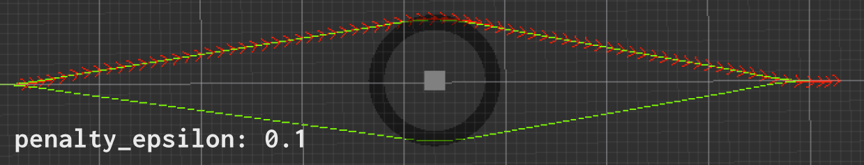
obstacle_association_force_inclusion_factor: 10.0 the obstacles that will be taken into account are those closer than min_obstacle_dist * factor, if legacy is false
obstacle_association_cutoff_factor: 40.0 the obstacles that are further than min_obstacle_dist * factor will not be taken into account, if legacy is false
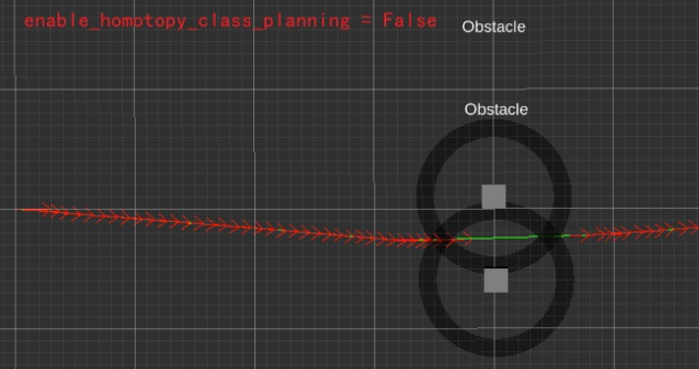
simple_exploration 默认false. 如果为true,不同的 trajectories are explored using a simple left-right approach (pass each obstacle on the left or right side) for path generation, otherwise sample possible roadmaps randomly in a specified region between start and goal.
ros::Time last_error = ros::Time::now(); std::string tf_error; //确保机器人global_frame_和robot_base_frame_之间的有效转换, 否则一直停留在这里阻塞 // 这里已经写死为 0.1,有需要可以改变 while (ros::ok() && !tf_.waitForTransform(global_frame_, robot_base_frame_, ros::Time(), ros::Duration(0.1), ros::Duration(0.01), &tf_error)) { ros::spinOnce(); // 如果5秒内未成功tf转换,报警 if (last_error + ros::Duration(5.0) < ros::Time::now()) { ROS_WARN("Timed out waiting for transform from %s to %s to become available before running costmap, tf error: %s", robot_base_frame_.c_str(), global_frame_.c_str(), tf_error.c_str()); last_error = ros::Time::now(); } // The error string will accumulate and errors will typically be the same, so the last // will do for the warning above. Reset the string here to avoid accumulation. tf_error.clear(); } //检测是否需要“窗口滚动”,从参数服务器获取以下参数 bool rolling_window, track_unknown_space, always_send_full_costmap; private_nh.param("rolling_window", rolling_window, false); private_nh.param("track_unknown_space", track_unknown_space, false); private_nh.param("always_send_full_costmap", always_send_full_costmap, false);
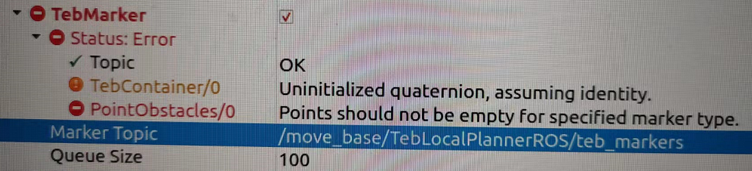
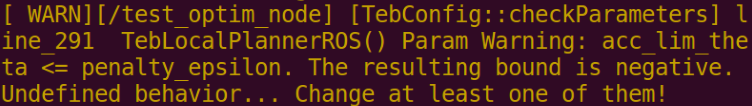
有时出现了下面的报错 这就是因为上面的0.1太小了
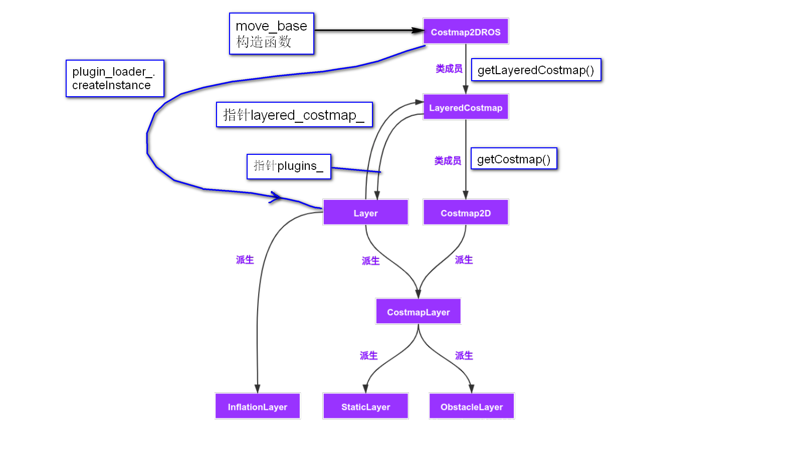
LayeredCostmap类的对象
layered_costmap_ = new LayeredCostmap(global_frame_, rolling_window, track_unknown_space);
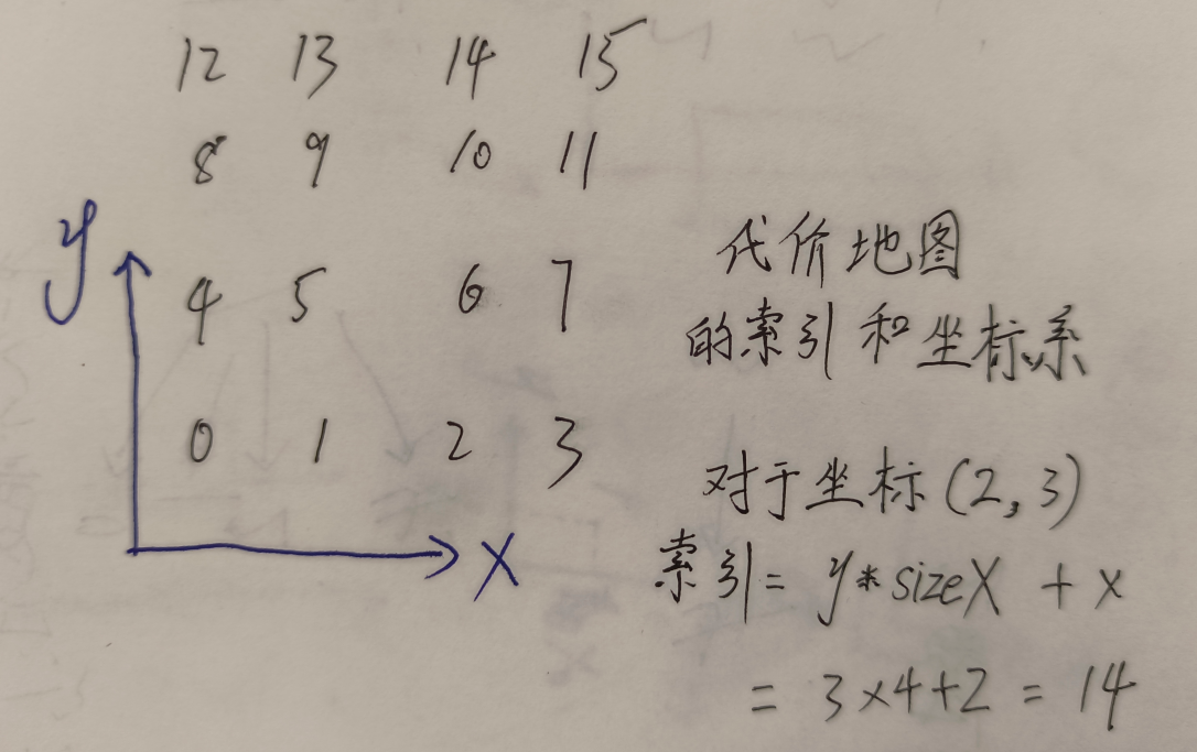
如果是局部代价地图,窗口边长4,分辨率0.05,那么窗口的像素边长就是80,这里的机器人的坐标 mx my 就在(40, 40)左右,因为它总在局部代价地图中心
1
2
3
4
5
if (!costmap_->worldToMap(x, y, mx, my)) { ROS_FATAL("The dimensions of costmap is too small to fully include robot's footprint"); return; } unsignedchar cost = costmap_->getCost(mx, my);