obstacle_cost_exponent和min_obstacle_dist的设置,一般都会进入if情况。 注意 max cost (before weighting) is the same as the straight line version and that all other costs are below the straight line (for positive exponent), so it may be necessary to increase weight_obstacle and/or the inflation_weight when using larger exponents.
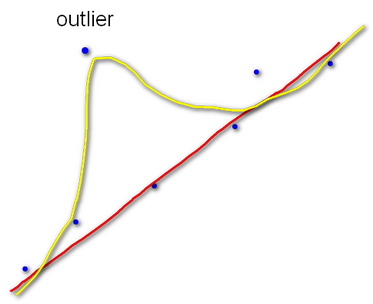
After running optimize() once, I am finding a high number of outliers. Is there any way to delete a single edge out of the graph and run optimize again, or do I have to construct it again?
The method removeEdge() removes the edge from a graph and unlinks it from all of the vertices it was attached to. After you call it on your edges, I think you need to call initializeOptimization() to reset all of g2o’s internal data structures to the new graph configuration. You should then be able to call optimize()
setLevel(int ) is useful when you call optimizer.initializeOptimization(int ). If you assign initializeOptimization(0), the optimizer will include all edges up to level 0 in the optimization, and edges set to level >=1 will not be included
CMake Deprecation Warning at CMakeLists.txt:1 (cmake_minimum_required): Compatibility with CMake < 2.8.12 will be removed from a future version of CMake
sed -i "s/2.8.3/3.19/g" `grep 2.8.3 -rl . --include="*.txt" `
这个命令不要滥用,否则可能更改过多
涉及PCL的一个警告
1 2 3 4 5
CMake Warning (dev) at /usr/local/share/cmake-3.17/Modules/FindPackageHandleStandardArgs.cmake:272 (message): The package name passed to `find_package_handle_standard_args` (PCL_KDTREE) does not match the name of the calling package (PCL). This can lead to problems in calling code that expects `find_package` result variables (e.g., `_FOUND`) to follow a certain pattern.
在find_package(PCL REQUIRED)之前加上
1 2 3
if(NOT DEFINED CMAKE_SUPPRESS_DEVELOPER_WARNINGS) set(CMAKE_SUPPRESS_DEVELOPER_WARNINGS 1 CACHE INTERNAL "No dev warnings") endif()
No rule to make target
有时明明写好了,但编译会出现报错,看上去是CMakeLists中没有编译规则
1 2 3 4 5 6
make[2]: *** No rule to make target 'package/CMakeFiles/test_bin.dir/build'。 停止。 CMakeFiles/Makefile2:3192: recipe for target 'package/CMakeFiles/test_bin.dir/all' failed make[1]: *** [package/CMakeFiles/test_bin.dir/all] Error 2 Makefile:138: recipe for target 'all' failed make: *** [all] Error 2 Invoking "make -j4 -l4" failed
此时再重新编译仍然报错,只要把CMakeLists改一下,再编译就通过了
CMakeCache 报错
执行编译时报错:
1
CMake Error: The current CMakeCache.txt directory /home/user/common/build/CMakeCache.txt is different than the directory /home/user/space/build where CMakeCache.txt was created. This may result in binaries being created in the wrong place. If you are not sure, reedit the CMakeCache.txt
要求是:标定板在激光正前方120°范围内,并且激光前方2m范围内只存在一个连续的直线线段,所以请在空旷的地方采集数据,不然激光数据会提取错误。需要充分旋转 roll 和 pitch。更直白一点,假设在长方形的标定板中心画了个十字线,那请绕着十字线的两个轴充分旋转,比如绕着竖轴旋转,然后还要绕着横轴旋转。在运行offline程序时,程序会将认为正确的直线会显示为红色。
Load apriltag pose size: 582 terminate called after throwing an instance of 'std::out_of_range' what(): vector::_M_range_check: __n (which is 18446744073709551615) >= this->size() (which is 57) [lasercamcal_ros-1] process has died
有时连录几次bag,都出现这种情况,估计是某个地方在for循环里push_back导致
结果不可观
计算初值阶段
1
2
3
4
5
6
7
8
9
~~~~~~~~~~~~~~~~~~~~~~~~~~~~~~~~~~~~~~~~~~~~~~~~~~ Notice Notice Notice: system unobservable !!!!!!! ~~~~~~~~~~~~~~~~~~~~~~~~~~~~~~~~~~~~~~~~~~~~~~~~~~
// Converts an Eigen Quaternion into a tf Matrix3x3. voidtf::matrixEigenToTF(const Eigen::Matrix3d &e, tf::Matrix3x3 &t) // Converts a tf Matrix3x3 into an Eigen Quaternion. voidtf::matrixTFToEigen(const tf::Matrix3x3 &t, Eigen::Matrix3d &e) // Converts an Eigen Affine3d into a tf Transform. voidtf::poseEigenToTF(const Eigen::Affine3d &e, tf::Pose &t) // Converts a tf Pose into an Eigen Affine3d. voidtf::poseTFToEigen(const tf::Pose &t, Eigen::Affine3d &e) // Converts an Eigen Quaternion into a tf Quaternion. voidtf::quaternionEigenToTF(const Eigen::Quaterniond &e, tf::Quaternion &t) // Converts a tf Quaternion into an Eigen Quaternion. voidtf::quaternionTFToEigen(const tf::Quaternion &t, Eigen::Quaterniond &e) // Converts an Eigen Affine3d into a tf Transform. voidtf::transformEigenToTF(const Eigen::Affine3d &e, tf::Transform &t) // Converts a tf Transform into an Eigen Affine3d. voidtf::transformTFToEigen(const tf::Transform &t, Eigen::Affine3d &e) // Converts an Eigen Vector3d into a tf Vector3. voidtf::vectorEigenToTF(const Eigen::Vector3d &e, tf::Vector3 &t) // Converts a tf Vector3 into an Eigen Vector3d. voidtf::vectorTFToEigen(const tf::Vector3 &t, Eigen::Vector3d &e)
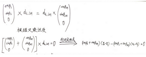
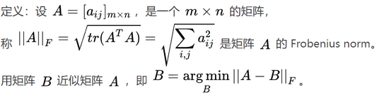
的推导过程](https://s2.loli.net/2023/03/04/UWQmsEB4AHIGSOr.png)