里程计是衡量我们从初始位姿到终点位姿的一个标准,通俗的说,要实现机器人的定位与导航,就需要知道机器人行进了多少距离,是往哪个方向行进的, odom的原点是机器人启动的位置。
里程计一个很重要的特性,是它只关心局部时间上的运动,多数时候是指两个时刻间的运动。当我们以某种间隔对时间进行采样时,就可估计运动物体在各时间间隔之内的运动。由于这个估计受噪声影响,先前时刻的估计误差,会累加到后面时间的运动之上
odom坐标系是在机器人运动前以当前观测到的数据建立的临时的坐标系,避免远离map原点而造成误差。比如轮子的编码器或者视觉里程计算法或者陀螺仪和加速度计。odom坐标系原则上是固定的,但可能会随着机器人的运动漂移,这就是累计误差,漂移导致odom不是一个很有用的长期的全局坐标,但是一个有用的短期坐标。在odom坐标系下机器人的位置必须是连续变化的,不能有突变和跳跃,比如人不能把机器人搬到其他地方。
里程计中也存在线速度角速度,但是这个线速度角速度是通过距离除以时间得到的,没有IMU的精确.
里程计的发布频率不能低,move_base里面默认订阅里程计的频率是20Hz,所以里程计至少也得20Hz,目前机器人的为50Hz
运动模型
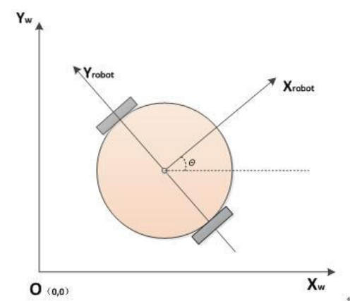
机器人的位置X,Y可以看做车在极小时间内的位置增量在X,Y方向的分量的积分。我们采用速度推算方式确定机器人的轨迹,在极小时间Δt内,以速度V移动的距离是Δd,分解到两坐标轴可以得到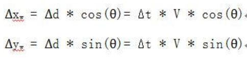
这样不断累积,就可以得到任意时间的位置: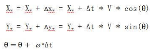
Δt是我们自己取的,比如10ms,可以在ROS中使用ros::Rate实现
V和ω并不是我们指定的速度,而是由指定速度和角速度根据航迹推演之后,分配到两个驱动轮上的速度Vl和Vr,再从硬件层根据Kinematics返回的速度Vx和ω。由于驱动轮不是全向轮,所以Vy是0
至于偏航角,有两种方法获取:编码器和IMU。编码器很依赖精度,效果不如IMU。使用IMU的话,θ就是其返回的偏航角Yaw,IMU上电时的Yaw为0,与小车航向一致,只是还要根据公式转换到
(-π,π]
tf关系
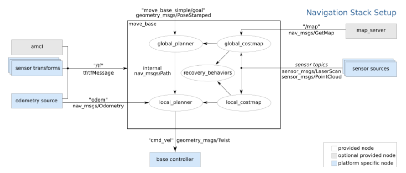
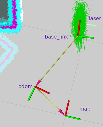
用到的tf父子关系为: map–>odometry–>base_link ,随着机器人的移动,我们需要生成机器人的里程计信息,如此可以提供机器在map中大致的位置,一般在一个节点里发出odometry->base_link的tf广播,它们的转换信息是每时每刻都在发布的。
odom的原点是机器人启动的位置,因为每次机器人启动的位置不同,所以一开始odom在map上的位置或转换矩阵是未知的,但是AMCL可以根据最佳粒子的位置推算出map->odom(就是说通过最佳粒子推算出机器人在地图的中的位置)的tf转换信息并发布到tf主题上,这样三者的tf父子关系就建立起来了,我们也就知道了base_link在map中的坐标。
不管机器人在哪启动,odom和map坐标系之间的tf理论上是不变的,发生的改变就是里程计的累计误差
一般来说map坐标系的坐标是通过传感器的信息不断的计算更新而来。比如激光雷达,视觉定位等等。因此能够有效的减少累积误差,但是也导致每次坐标更新可能会产生跳跃。map坐标系是一个很有用的长期全局坐标系。但是由于坐标会跳跃改变,这是一个比较差的局部坐标系(不适合用于避障和局部操作)。
map->odom变换代表了对里程计误差的纠正
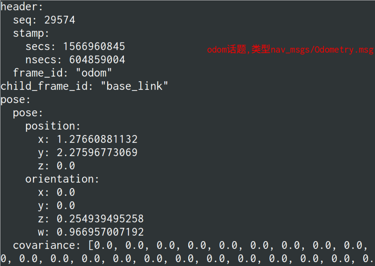
odom话题
odom消息成员:1
2
3
4std_msgs/Header header
string child_frame_id
geometry_msgs/PoseWithCovariance pose
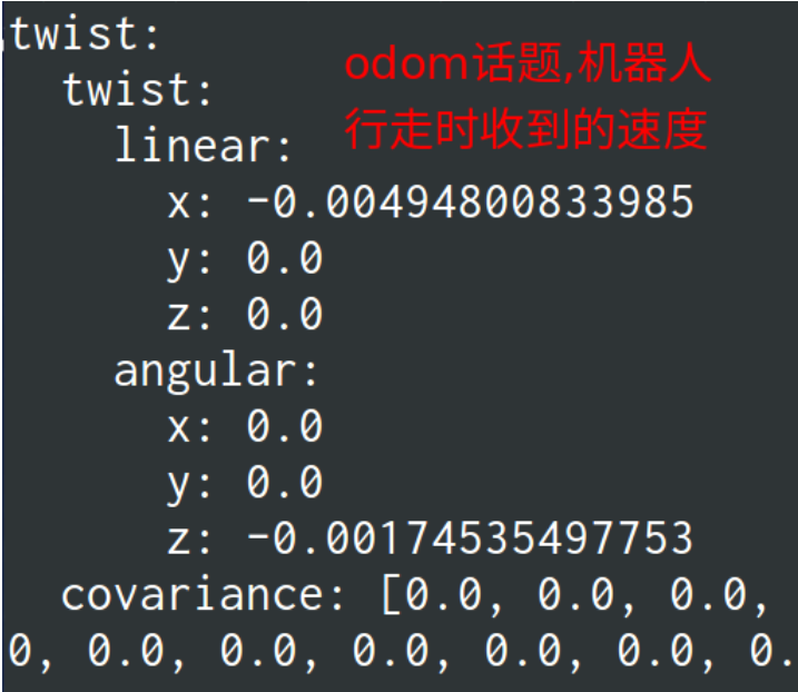
geometry_msgs/TwistWithCovariance twist
里程计向局部路径规划器传递当前机器人的速度,消息中的速度也在TrajectoryPlannerROS对象中的代价地图包含的robot_base_frame参数表示的坐标系中,一般就是base_link,这个参数是在全局代价地图的yaml文件中。
在rviz中添加Odometry,最好去掉它的Covariance项后面的勾,也就是在Odometry显示中不启用Covariance信息,否则将导致显示效果很难看
代码如下,对不同的机器人,获取线速度和角速度的方法不同,这里没有用到IMU1
2
3
4
5
6
7
8
9
10
11
12
13
14
15
16
17
18
19
20
21
22
23
24
25
26
27
28
29
30
31
32
33
34
35
36
37
38
39
40
41
42
43
44
45
46
47
48
49
50
51
52
53
54
55
56
57
58
59
60
61
62
63
64
65
66
67
68
69
70
71
72
73
74
75
76
77
78
79
80
81
82
83
static ros::Publisher *odomPubPtr;
double x = 0;
double y = 0;
double theta = 0;
ros::Time current_time;
ros::Time last_time;
geometry_msgs::TransformStamped odom_trans;
nav_msgs::Odometry odom;
void callback(const geometry_msgs::TwistConstPtr& velocity)
{
static tf::TransformBroadcaster odom_broadcaster;
double vx, vy, omega;
current_time = ros::Time::now();
vx = velocity->linear.x;
omega = velocity->angular.z;
//compute odometry in a typical way given the velocities of the robot
double dt = (current_time - last_time).toSec();
double delta_x = (vx * cos(theta) - vy * sin(theta)) * dt;
double delta_y = (vx * sin(theta) + vy * cos(theta)) * dt;
double delta_th = omega * dt;
x += delta_x;
y += delta_y;
theta += delta_th;
//since all odometry is 6DOF we'll need a quaternion created from yaw
geometry_msgs::Quaternion odom_quat = tf::createQuaternionMsgFromYaw(theta);
odom_trans.header.stamp = current_time;
odom_trans.transform.translation.x = x;
odom_trans.transform.translation.y = y;
odom_trans.transform.translation.z = 0.0;
odom_trans.transform.rotation = odom_quat;
odom_broadcaster.sendTransform(odom_trans);
odom.header.stamp = current_time;
//set the position
if(fabs(x) < 0.0001 ) x=0;
if(fabs(y) < 0.0001 ) y=0;
odom.pose.pose.position.x = x;
odom.pose.pose.position.y = y;
odom.pose.pose.position.z = 0.0;
odom.pose.pose.orientation = odom_quat;
odom.twist.twist.linear.x = vx;
odom.twist.twist.linear.y = vy;
odom.twist.twist.angular.z = omega;
odomPubPtr->publish(odom);
ROS_INFO_ONCE(" 开始发布里程计信息 ");
last_time = current_time;
}
int main(int argc, char** argv)
{
ros::init(argc, argv, "odometry_publisher");
ros::NodeHandle n;
setlocale(LC_ALL,"");
last_time = ros::Time::now();
odom_trans.header.frame_id = "odom";
odom_trans.child_frame_id = "base_link";
odom.header.frame_id = "odom";
odom.child_frame_id = "base_link";
ros::Subscriber sub = n.subscribe<geometry_msgs::Twist>("velocity",20,callback);
ros::Publisher odom_pub = n.advertise<nav_msgs::Odometry>("odom", 50);
odomPubPtr = &odom_pub;
ros::spin();
}
这里的里程计频率就由话题velocity的频率决定了,因为是订阅建立后阻塞了,回调函数就一直执行
如果像这样写,每次都要通过网络获取话题的消息,会明显降低里程计的频率1
2
3
4
5
6
7
8
9
10boost::shared_ptr<geometry_msgs::Twist const> velEdge; // 必须有const
velEdge = ros::topic::waitForMessage<geometry_msgs::Twist>("velocity",ros::Duration(1));
if(velEdge != NULL)
{
velocity = *velEdge;
vx = velocity.linear.x;
omega = velocity.angular.z;
}
else
ROS_WARN("linear and angular velocity not received !");