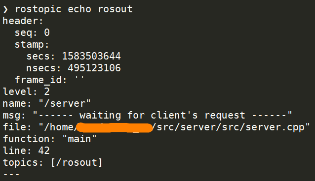
在ros中,我们有时需要一次性启动多个节点,这种情况下再用rosrun就力不从心了,于是出现了roslaunch命令和launch文件,launch文件使用XML语法launch文件使用XML语法。roslaunch不保证节点开始的顺序。因为没有办法从外部知道节点何时被完全初始化,所以所有被启动的节点必须是robust,以便以任何顺序启动。
node
node的形式为:1
<node name="node-name" pkg="pkg-name" type="executable-name" output="screen" />
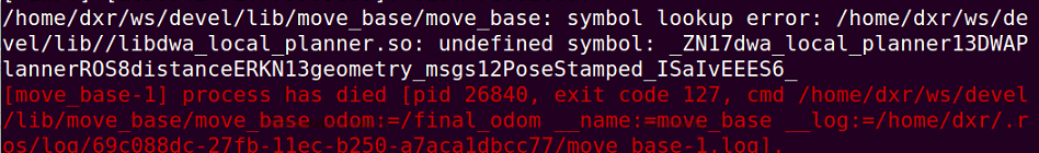
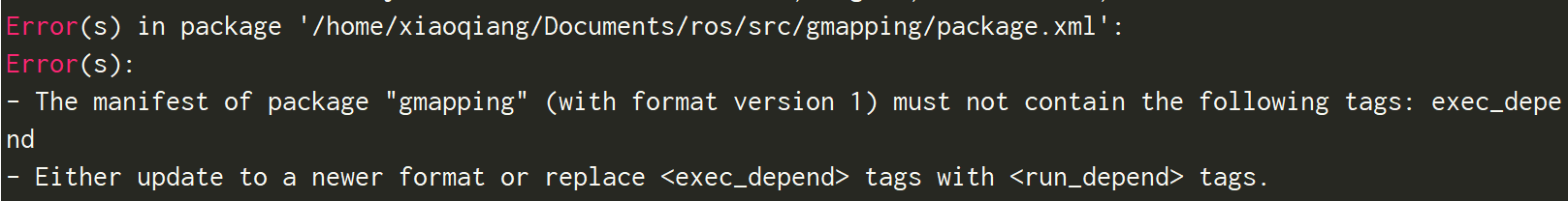
node的三个属性分别为节点名字(name)、程序包名字(pkg)和可执行文件(type)的名字。尤其注意:type是CMakeLists中的add_executable中的名称,而不是cpp文件的名称。 否则会报错:
不要把pkg写成 pkg="$(find package)",可能会报错:1
2ERROR: cannot launch node of type [path_to_file] package_path
ROS path [0]=/opt/ros/...
name属性给节点指派了名称,它将覆盖任何通过调用ros::init来赋予节点的名称。另外node标签内也可以用过arg设置节点参数值。如果node标签有children标签,就需要显式标签来定义。即末尾为/node>
当roslaunch开启所有nodes后,roslaunch会监视每个node,记录那些仍然活动的nodes。对于每个node,当其终止后,我们可以要求roslaunch重启该node,通过使用respawn属性。通过使用respawn属性: respawn="true"
respawn_delay="10"会让节点终止后,隔一段时间重新运行,和respawn="true"同时使用,单位秒
多个同样的节点有不同的topic
在launch文件中使用node_1和node_2,它们的type是一样的,但是还发布了话题。这样启动launch就会出现两个节点同一个话题的情况,这不是我们想要的。 此时要在代码中对NodeHandle的构造函数加~,这时param也加上了节点名做前缀,可能还要在launch中用remap修改话题名。
param
param是ROS系统运行中的参数,存储在参数服务器中。在launch文件中通过元素加载参数;launch文件执行后,参数就加载到ROS的参数服务器上了。每个活跃的节点都可以通过 ros::param::get()或getParam接口来获取parameter的值,用户也可以在终端中通过rosparam命令或获得参数的值。
<param>的使用方法如下:1
<param name="frame" type="string" value="odom"/> <!-- type可以没有 -->
1 | string f; |
argument
argument是另外一个概念,类似于launch文件内部的局部变量,仅限于launch文件使用,和ROS节点内部的实现没有关系。argument只在启动文件内才有意义,不能被节点直接获取的
设置argument使用1
2<arg name="arg-name" default="arg-value" />
<arg name="arg-name" default="arg-unchanged-value" />
launch文件中需要使用到argument时,可以使用如下方式调用:1
2
3<arg name="arg-name" default="arg-value" />
<param name = "foo" value="$(arg arg-name)" />
<node name="node" pkg="package" type="type "args="$(arg arg-name)" />
也就是不能直接在程序里获得arg的值,只能通过param来间接获得。不过在读move_base.cpp时发现,如果main函数带有argc和argv,那么arg参数值实际就是argv[1],也就是ros运行时是以node_name arg-value的形式进行的
1 | int main(int argc, char **argv) |
虽然在launch文件中规定了参数的值,但我们在终端使用roslaunch命令时,还可以修改这个值,但前提是arg的赋值是用default,不是用value,命令如下:1
roslaunch package-name launch-file-name arg-name:=arg-value
注意是 arg-name ,不是name
标签
使用这个标签可以读取bashrc里的环境变量没有关系,也就是说 在roslaunch里获取 bashrc 里的环境变量 。 除此之外看不出跟arg参数还有什么区别。
我们常常遇到一种情况:多个launch都用到一个参数,比如某个路径,如果用arg,只能在每个launch里设置它,或者在一个单独launch里设置好,然后所有launch都去include这个launch。 如果有了环境变量,就可以在每个launch里直接使用这个环境变量代表的路径了。1
2<param name="path1" value="$(env PATH1)" />
<param name="path2" value="$(env PATH2)" />
eval
$(eval <expression>)可以实现复杂的python表达式,不太常用
例如:1
2
3<param name="circumference" value="$(eval 2.* 3.1415 * arg('radius'))"/>
<!-- 当前launch所在的路径 -->
<arg name="abspath" value="$(eval eval('_' + '_import_' + '_(\'os\').path.abspath(\'.\')') )" />
launch中加条件判断
launch文件部分如下:1
2
3
4
5
6
7<arg name="driver_enable" default="true"/>
<group if="$(arg driver_enable)">
<include file= "$(find openni2_launch)/launch/openni2.launch"/>
</group>
其实还是从上一节引申而来,在终端使用如下命令,根据arg的值是否执行,:1
roslaunch [pkg] [node] driver_enable:=false
如果是false,就不加载openni2.launch
include另一个launch
在launch文件中可以include另一个launch文件,扩展名也可以是xml1
<include file="$(find package)/launch/amcl.launch"/>
一般这样写,package的路径用shell命令 $(find package)获得
其他
roslaunch中的可选标签:
- ns = foo(可选) 在”foo”命名空间中启动节点
clear_params = true 或 false 在启动前删除节点的私有命名空间中的所有参数。
master 目前已经淘汰, master 用以配置 ROS Master
restart 或 no. defines the behavior for starting a new master with the roslaunch session.
- 如果是
start, then a master will be started if none is running. - 如果是
restart, then a fresh master will be started for the demo — any existing master will be shutdown first. - 默认是
no, which is to do nothing.
launch-prefix
launch-prefix=”nice” : nice your process to lower its CPU usage
launch-prefix=”screen -d -m gdb —args” : useful if the node is being run on another machine; you can then ssh to that machine and do screen -D -R to see the gdb session
required
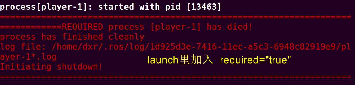
这个可加可不加,加了之后在关闭时会有这样的提示
参考: 如何多次启动相同名称的节点